Causal Inference Series (I)
0. 前言
Causal Inference (因果推断) 已经在多个领域发挥出巨大作用, 尽管早已经听说过其大名, 但是从未步入这个领域好好学习一番, 通常是浅尝辄止. 为此在博客开一个系列, 一是用于记录学习, 二是希望能够起到监督作用…
由于是入门学习, 因此课程和书籍选择了相对简单的. 根据网上的推荐和实际体验, 感觉 Brady Neal 的系列介绍比较合适, 因此这个系列都将会以 Brady Neal 的课程为基础. 课程链接: https://www.bradyneal.com/causal-inference-course
由于这是个人学习笔记, 我作为初学者, 在博客中记录的内容和理解难免会有错误. 希望各位能够指正, 并请不吝赐教, 在下将不胜感激.
1. 第一章 Motivation: Why You Might Care
第一章主要介绍辛普森悖论, 以及向我们初步展示相关性和因果性的联系与区别.
1.1 Simpson’s Paradox
通常因果推断的第一课都是 Simpson’s Paradox (辛普森悖论) . 它说了这么一件事 : 假设现在有种病, 我们有 2 个治疗方案, treatment A and treatment B. 在做实验的时候, treatment B 比较稀缺, 只有较少的志愿者可以用上 B, 比如 treatment A and treatment B 的志愿者分别为 73% 和 27% . 现在得到这么一组数据 :
表中, 百分比指的是接受相应的 treatment 后志愿者死亡率. Mild组 表示病的不重 , Severe组 表示病的比较严重.
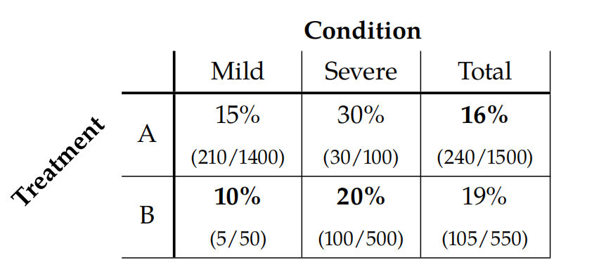
从上表可以看到, 无论是哪个分组, 明显 treatment B 死亡率更低. 但是有趣的是, 当你纵观所有人, 即 Total 列反而是 treatment A 死亡率更低. 那么到底哪个 treatment 更好呢?
上表有个关键的问题, 总共 550 个人 接受了 treatment B, 但是有 500 个是重病患者. 因此计算最终的死亡率时候, 重病死亡率的权重更大, 导致对于 treatment B 的 Total 死亡率接近 20 %. 同理, 对于 treatment A, 轻症患者更多, 所以最后的平均死亡率反而比较低. 所以, 到底哪个更好?? 实际上, 这个答案是基于因果关系的.
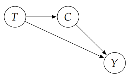
如果受试者的 Condition 影响 treatment. 举个例子, 医生会根据患病情况来给出 treatment, 如果患病情况比较轻, 那么通常会安排 treatment A. 反之, 病重的会安排 treatment B. 他们之间的关系如下:

那这时, 这需要看不同患病情况下, treatment 的治愈率, 显然这种情况下 treatment B 更好.
如果受试者的 treatment 影响 Condition. 举个例子, 比如 treatment B 比较牛逼但是稀缺, 本来患病了就直接用药即可, 但是由于人们非要等着 treatment B 导致病情恶化. 当然对于 treatment A 是没有这个问题的. 那么这是他们的关系就是:
此时, 显然尽管 treatment B 药效好, 但是为了存活率, 我们应该选择 treatment A. 总的来说, 当我们有了因果关系之后, 就可以解决 Simpson’s Paradox 了.
1.2 Correlation Does Not Imply Causation
这是一个很关键的思想: $相关性 \neq 因果性$. 有个”Nicolas Cage and Pool Drownings”的例子, 说的是演员尼古拉斯凯奇和发生游泳溺水次数的相关性.
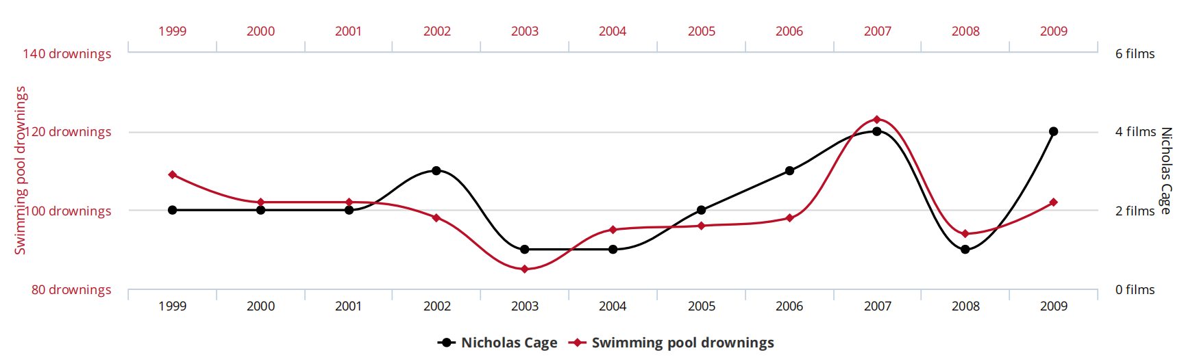
有人发现, 你用这个哥们儿出演电影次数和有人游泳溺水次数算线性相关性, 结果可能显示高度相关, 这明显是很离谱的事情. 显然他们并没有什么因果性.
再看一个例子, 人们发现一个事情, 那些晚上很晚回来并且穿着鞋子睡觉的人, 第二天早上醒来会头痛. 事实确实发生了, 人们会说他们是相关的. 但是实际隐藏了一个条件, 这些晚上穿着鞋子睡觉的人, 大概率是喝酒喝醉了回来倒头就睡, 第二天头疼也八成是因为喝酒喝的. 我们称背后隐藏的这个条件为 “confounder”.
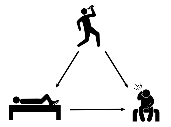
我们称 confounder 与 研究对象 的关联为 “confounding association” . 如果想单纯探究 “穿鞋睡觉 -> 第二天头疼” 的因果关系, 我们就必须先断掉 confounder 的影响.
2. 第二章 Potential Outcomes
第二章主要介绍基础概念.
2.1 Potential Outcomes and Individual Treatment Effects
考虑一个例子:假设有个人心情不太好,有人想送给他一只狗.如果他接受了这只狗,那他可能会变得开心.但如果他拒绝了呢?他会不会继续感到不高兴呢?反过来想,如果他接受了这只狗,但他仍然感到不高兴,那么我怎么知道,如果不送给他,他是否会变得更开心呢?
2.1.1 Potential Outcomes
根据前面的分析,实际上针对某个人采取不同的处理方式会产生不同的结果,这是一个潜在的结论.我们在之后的讨论中, 称这个潜在的输出为 $\mathit {Y}$ .
在上边的例子中, $\mathit {Y} = 1$ 表示高兴, $\mathit {Y} = 0$ 为不高兴.
用 $\mathit {T}$ 表示 treatment 这个随机变量. $\mathit {T} = 1$ 表示接受狗子, $\mathit {T} = 0$ 表示不接受.
使用 $\mathit {Y(1)}$ 表示接受狗子以后的潜在输出, $\mathit {Y(0)}$ 为采取不接受狗子后的输出.
2.1.2 Individual Treatment Effects
因为有很多人, 我们使用 $\tau_i \triangleq Y_i(1) - Y_i(0)$ 来评估某个个体采取 treatment 之后的潜在输出结果.
你可以观察接受狗子之后, 观察 $\mathit {Y(1)}$. 反之, 你可以不接受狗子来观察 $\mathit {Y(0)}$. 但是你不能同时观察到 $\mathit {Y(1)}$ 和 $\mathit {Y(0)}$ !!!! 这个问题就是 “Fundamental Problem of Causal Inference”
2.2 Average Treatment Effects
因为每个人可能有些许差异, 实际要想客观的评估 treatment 的作用, 我们要对所有人求 treatment 期望:
\[\tau \triangleq \mathbb{E}[Y_i(1) - Y_i(0)] = \mathbb{E}[Y(1) - Y(0)]\]但是上式由于 Fundamental Problem of Causal Inference, 实际上比较难做到计算. 参看下表:
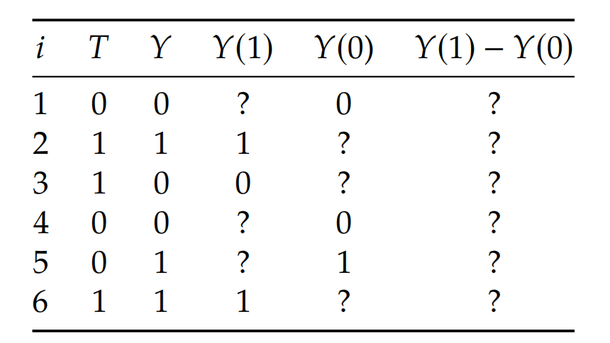
当对个体 $i$ 采取了 treatment 0 的时候, 你只能观察到 $Y_i(0)$, 观察不到 $Y_i(1)$. 也就是说以下式子不成立:
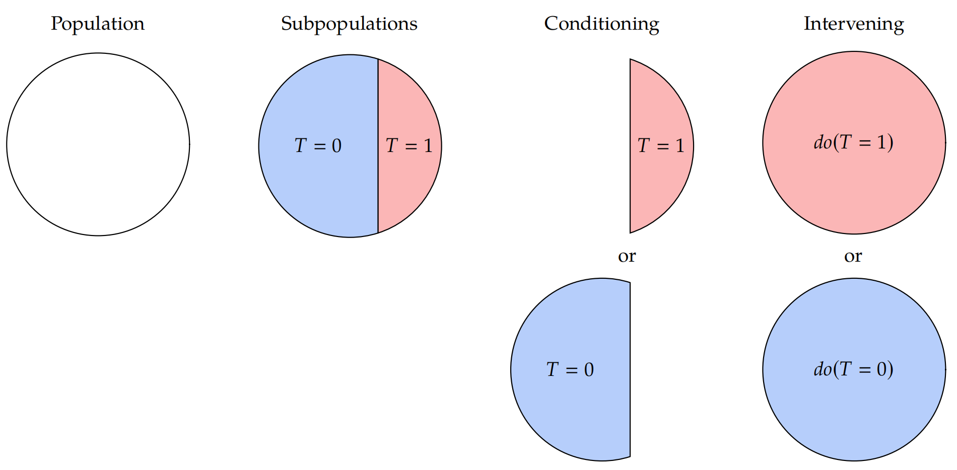
\[\mathbb{E}[Y(1) - Y(0)] = \mathbb{E}[Y(1)] - \mathbb{E}[Y(0)] \neq \mathbb{E}[Y(1) | T = 1 ] - \mathbb{E}[Y(0) | T = 0]\]可以看到, treatment 0 对应的集合只是一部分, 不能作为全部的结果, $\mathbb{E}[Y(1)]$ 理应是最右边的结果(Intervening).
2.2.1 Ignorability and Exchangeability
那么什么时候, 或者基于什么假设, 上式能够成立呢?
Assumption 2.1 Ignorability / Exchangeability
\[(Y(1) , Y(0)) \amalg T\]
当假设满足 Ignorability 的时候, 能够做到以下式子成立. 这里 Ignorability 指的是, 可以忽视缺失的数据.
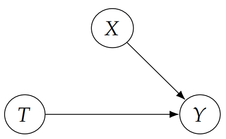
\[\begin{aligned} \mathbb{E}[Y(1) - Y(0)] &= \mathbb{E}[Y(1)] - \mathbb{E}[Y(0)] \newline &=\mathbb{E}[Y(1) \mid T = 1 ] - \mathbb{E}[Y(0) \mid T = 0] \ (Ignorability) \newline &=\mathbb{E}[Y \mid T = 1 ] - \mathbb{E}[Y \mid T = 0] \ (之后讨论) \end{aligned}\]上式表明 Y(1) 就只基于 T = 1 , 不受其他影响 , 即没有 confounder 的影响了. 如图:
这个假设也叫 Exchangeability, 表示说 $\mathbb{E}[Y(0) \mid T = 0] = \mathbb{E}[Y(0) \mid T = 1] = \mathbb{E}[Y(0) \mid t ]$ , 这其实就是说对于 group A 或者 group B, 把他们交换 treatment group 和 control group, 输出的结果只与 treatment 有关, 和 group A 或者 group B 没有关系 (尤其是 confounder). 也暗示着除了 treatment 的方式有区别, 不受其他影响.
Definition 2.1 Identifiability
causal quantity (e.g. $\mathbb{E}[Y(t)]$) is Identifiable if we can compute it from a purely statistical quantity (e.g. $\mathbb{E}[Y \mid t]$)
这个 Identifiability 是说, 我们可以用 $\mathbb{E}[Y \mid t]$ 代替 $\mathbb{E}[Y(t)]$.
2.2.2 Conditional Exchangeability and Unconfoundedness
实际中, 我们直接假设 group A 或者 group B 除了 treatment 的方式有区别, 不受其他影响. 但是这个不太现实, 明显是不合理的. 但是我们考虑, 如果可以控制一些条件, 让他们除了 treatment 方式有区别, 其他没有区别.
Assumption 2.2 Conditional Exchangeability / Unconfoundedness
\[(Y(1) , Y(0)) \amalg T \mid X\]
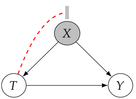
当假设满足 Conditional Exchangeability 的时候, 换句话说, 我们控制了 confounder X, 使得 group 基于同样的 confounder , 那这时去做 treatment, 就实现了 treatment 直接作用于 outcome, 不会因为潜在的 confounder 影响 outcome. 如图所示:

于是有以下公式成立:
\[\begin{aligned} \mathbb{E}[Y(1) - Y(0) \mid X] &= \mathbb{E}[Y(1) \mid X] - \mathbb{E}[Y(0) \mid X] \newline &=\mathbb{E}[Y(1) \mid T = 1, X] - \mathbb{E}[Y(0) \mid T = 0, X] \ (Ignorability) \newline &=\mathbb{E}[Y \mid T = 1, X ] - \mathbb{E}[Y \mid T = 0, X] \ (fix confounder) \end{aligned}\]则:
\[\begin{aligned} \mathbb{E}[Y(1) - Y(0) ] &= \mathbb{E}_X[\mathbb{E}[Y(1) \mid X] - \mathbb{E}[Y(0) \mid X]] \newline &=\mathbb{E}_X[\mathbb{E}[Y(1) \mid T = 1, X] - \mathbb{E}[Y(0) \mid T = 0, X]] \ (Ignorability) \newline &=\mathbb{E}_X[\mathbb{E}[Y \mid T = 1, X ] - \mathbb{E}[Y \mid T = 0, X] ]\ (expect \ confounder) \end{aligned}\]Conditional exchangeability (Assumption 2.2) is a core assumption for causal inference and goes by many names. For example, the following are reasonably commonly used to refer to the same assumption: unconfoundedness, conditional ignorability, no unobserved confounding, selection on observables, no omitted variable bias, etc.
$\textit{We will use the name “unconfoundedness” a fair amount throughout this book.}$
Theorem 2.1 (Adjustment Formula) Given the assumptions of unconfoundedness, positivity, consistency, and no interference, we can identify the average treatment effect:
\[\mathbb{E}[Y(1) - Y(0) ] = \mathbb{E}_X[\mathbb{E}[Y \mid T = 1, X ] - \mathbb{E}[Y \mid T = 0, X] ]\]
不过上述的式子还是有缺陷, 我们只是理想的假设 fixed confounder 是全部的, 但很多 confounder 都是潜在未知的, 我们实际不能保证 fix 住的 confounder 就是全部的, 这就会导致还是会有从 treatment -> confounder -> outcome 这条链路的影响存在.